Binary Classification

Looking to classify $y \in \{0,1\}$, a binary outcome.

Example (Tumour Classification)

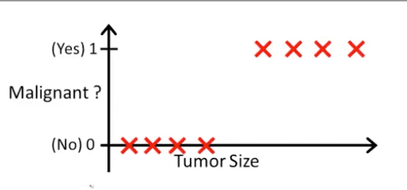
In an example like this, we could try using linear regression and use a threshold classifier such as:

• If $h_0 (x) \geq 0.5$, predict $y=1$
• If $h_0(x) < 0.5$, predict $y=0$

However, outlier points which can skew the regression line gives us a worse hypothesis. For this reason, linear regression isn’t fantastic for binary classification.

Linear regression can also allow values to extend beyond the range $\{0,1\}$, again making it a weak model for binary classification.

Introducing Logistical Regression

For this type of model, we want:

$0 \leq g_\theta (x) \leq 1$

For this reason, we will need to change our definition of $h_\theta (x)$ from what was used in linear regression. Our new hypothesis will be defined as:

$h_\theta (x) = g(\theta^T x), \quad g(z) = \frac{1}{1+e^{-z}}$

Where $g(z)$ can be referred to as the Sigmoid or Logistic function. The full version of our hypothesis function is:

$h_\theta (x) = \frac{1}{1+e^{-\theta ^Tx}}$

As before, we want to fit the parameters $\theta$.

Interpretation of Hypothesis

When $h_\theta (x)$ outputs a number, we will interpret it as the estimated probability that $y=1$ on input $x$.

For example, if we are using the tumour example with:

$x = \begin{bmatrix} x_0 \\ x_1 \end{bmatrix} = \begin{bmatrix} 1 \\ \text{Tumour Size} \end{bmatrix}, \quad h_\theta (x) = 0.7$

i.e. the probability of $y=1$ is $0.7$. Then we say that the patient has a $70\%$ chance of the tumour being malignant. More formally, we can write this as:

$h_\theta (x) = \Pr(y=1 | x;\theta)$

Since $y$ can only be either $0$ or $1$, we can also compute the probability that $y=0$

Decision Boundary

For logistic regression, we will define our hypothesis decision boundary as:

• Predict $y=1$ if $h_\theta (x) \geq 0.5$
• Predict $y=0$ if $h_\theta (x) < 0.5$

When will we end up in such cases? If we look at the sigmoid function:

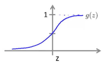
• $h_\theta (x) \geq 0.5$ when $\theta^T x\geq 0$
• $h_\theta (x) < 0.5$ when $\theta^Tx < 0$

Example

Consider the following dataset:

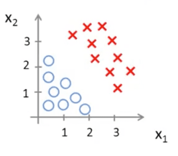
Our hypothesis would therefore be:

$h_\theta (x) = g(\theta_0 + \theta_1 x_1 + \theta_2 x_2)$

Further suppose that our fitted values of theta are:

$\theta = \begin{bmatrix}-3 \\ 1\\1\end{bmatrix}$

In this case, we will predict $y=1$ if:

$\begin{aligned} -3 + x_1 + x_2 &\geq 0\\ x_1 + x_2 &\geq 3 \end{aligned}$

Which is an equation for the following decision boundary line:

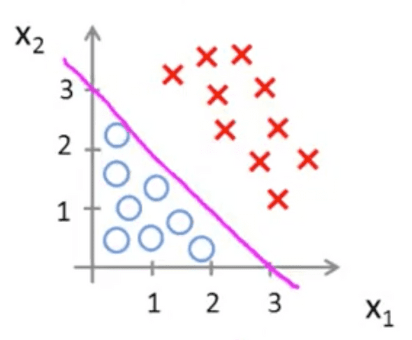
Therefore, we will predict $y=1$ for any point that falls to the right of the line. Vice-versa for $y=0$.

Non-linear Decision Boundary

Consider the following dataset:

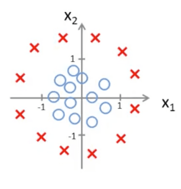
In linear regression, we were able to add higher order polynomials for situations like this. We can do the same with logistic regression. Suppose our hypothesis looks like:

$h_\theta (x) = g(\theta_0 + \theta_1 x_1 + \theta_2 x_2 + \theta_3 x_1 ^2 + \theta_4 x_2 ^2)$

Futher suppose that our fitted values are:

$\theta = \begin{bmatrix} -1\\0\\0\\1\\1\end{bmatrix}$

Therefore, we predict $y=0$ if:

$\begin{aligned} -1 + x_1 ^2 + x_2 ^2 &\geq 0\\ x_1 ^2 + x_2 ^2 &\geq 1 \end{aligned}$

This produces the following decision boundary:

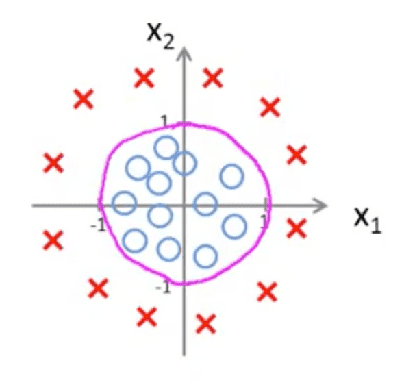
You can use polynomial terms to fit decision boundaries that take on many different shapes and sizes, not just circles.

Built with GatsbyJS